OpenFlights Analysis with grafeoR
Source:vignettes/openflights-analysis.Rmd
openflights-analysis.RmdThe package ships with a compact real-world OpenFlights subset so you can test the Rust binding against graph data that looks like an actual transport network, not just toy nodes and edges.
The bundled sample contains:
- the 20 airports with the highest outbound route counts in the upstream OpenFlights snapshot
- the 1,129 airline route records whose source and destination are both inside that 20-airport subset
sample <- openflights_sample_data()

dim(sample$airports)
#> [1] 20  7
dim(sample$routes)
#> [1] 1129    5
head(sample$airports[, c("iata", "city", "country", "snapshot_outbound_routes")])
#>   iata      city        country snapshot_outbound_routes
#> 1  ATL   Atlanta  United States                      915
#> 2  ORD   Chicago  United States                      558
#> 3  PEK   Beijing          China                      535
#> 4  LHR    London United Kingdom                      527
#> 5  CDG     Paris         France                      524
#> 6  FRA Frankfurt        Germany                      497
head(sample$routes)
#>   airline source_iata dest_iata stops equipment
#> 1      DL         AMS       ATL     0   333 76W
#> 2      KL         AMS       ATL     0       777
#> 3      HV         AMS       BCN     0   73H 73W
#> 4      IB         AMS       BCN     0       320
#> 5      KL         AMS       BCN     0       737
#> 6      MU         AMS       BCN     0       737
Load the graph into Grafeo
gql_string <- function(x) {
  if (is.null(x) || is.na(x)) {
    return("NULL")
  }

  value <- gsub("\\\\", "\\\\\\\\", as.character(x), perl = TRUE)
  value <- gsub("\"", "\\\\\"", value, fixed = TRUE)
  paste0("\"", value, "\"")
}

load_openflights_graph <- function(db, sample) {
  tx <- db$begin()
  on.exit(
    if (tx$is_active()) {
      try(tx$rollback(), silent = TRUE)
    },
    add = TRUE
  )

  for (i in seq_len(nrow(sample$airports))) {
    row <- sample$airports[i, ]
    tx$execute(sprintf(
      paste0(
        "INSERT (:Airport {",
        "iata: %s, name: %s, city: %s, country: %s, ",
        "lat: %.6f, lng: %.6f, snapshot_outbound_routes: %d",
        "})"
      ),
      gql_string(row$iata),
      gql_string(row$name),
      gql_string(row$city),
      gql_string(row$country),
      row$latitude,
      row$longitude,
      as.integer(row$snapshot_outbound_routes)
    ))
  }

  for (i in seq_len(nrow(sample$routes))) {
    row <- sample$routes[i, ]
    tx$execute(sprintf(
      paste0(
        "MATCH (src:Airport {iata: %s}), (dst:Airport {iata: %s}) ",
        "INSERT (src)-[:ROUTE {airline: %s, stops: %d, equipment: %s}]->(dst)"
      ),
      gql_string(row$source_iata),
      gql_string(row$dest_iata),
      gql_string(row$airline),
      as.integer(row$stops),
      gql_string(row$equipment)
    ))
  }

  tx$commit()
  invisible(db)
}
db <- grafeo_db()

load_openflights_graph(db, sample)
db$info()
#> $graph_model
#> [1] "LPG"
#>
#> $node_count
#> [1] 20
#>
#> $edge_count
#> [1] 1129
#>
#> $is_persistent
#> [1] FALSE
#>
#> $path
#> NULL
#>
#> $wal_enabled
#> [1] FALSE
#>
#> $version
#> [1] "0.5.23"
#>
#> $current_graph
#> NULL
Query airport and route data back into R
For the charts below, grafeoR is used to pull nodes and
edges back into R as data frames, and the aggregation for plotting is
handled on the R side.
airports_tbl <- db$query(
paste(
"MATCH (a:Airport)",
"RETURN a.iata, a.name, a.city, a.country, a.lat, a.lng,",
"a.snapshot_outbound_routes",
"ORDER BY a.snapshot_outbound_routes DESC, a.iata"
)
)
routes_tbl <- db$query(
paste(
"MATCH (src:Airport)-[r:ROUTE]->(dst:Airport)",
"RETURN src.iata, src.lat, src.lng, dst.iata, dst.lat, dst.lng, r.airline"
)
)
route_segments <- aggregate(
routes_tbl$r.airline,
by = list(
source_iata = routes_tbl$src.iata,
source_lat = routes_tbl$src.lat,
source_lng = routes_tbl$src.lng,
dest_iata = routes_tbl$dst.iata,
dest_lat = routes_tbl$dst.lat,
dest_lng = routes_tbl$dst.lng
),
FUN = length
)
names(route_segments)[names(route_segments) == "x"] <- "airline_count"
route_segments <- route_segments[
order(
-route_segments$airline_count,
route_segments$source_iata,
route_segments$dest_iata
),
,
]
head(airports_tbl[, c("a.iata", "a.city", "a.country", "a.snapshot_outbound_routes")])
#> a.iata a.city a.country a.snapshot_outbound_routes
#> 1 ATL Atlanta United States 915
#> 2 ORD Chicago United States 558
#> 3 PEK Beijing China 535
#> 4 LHR London United Kingdom 527
#> 5 CDG Paris France 524
#> 6 FRA Frankfurt Germany 497
head(route_segments)
#> source_iata source_lat source_lng dest_iata dest_lat dest_lng
#> 55 ORD 41.9786 -87.904800 ATL 33.6367 -84.428101
#> 40 ATL 33.6367 -84.428101 ORD 41.9786 -87.904800
#> 69 ATL 33.6367 -84.428101 MIA 25.7932 -80.290604
#> 98 JFK 40.6398 -73.778900 LHR 51.4706 -0.461941
#> 81 LHR 51.4706 -0.461941 JFK 40.6398 -73.778900
#> 56 MIA 25.7932 -80.290604 ATL 33.6367 -84.428101
#> airline_count
#> 55 20
#> 40 19
#> 69 12
#> 98 12
#> 81 12
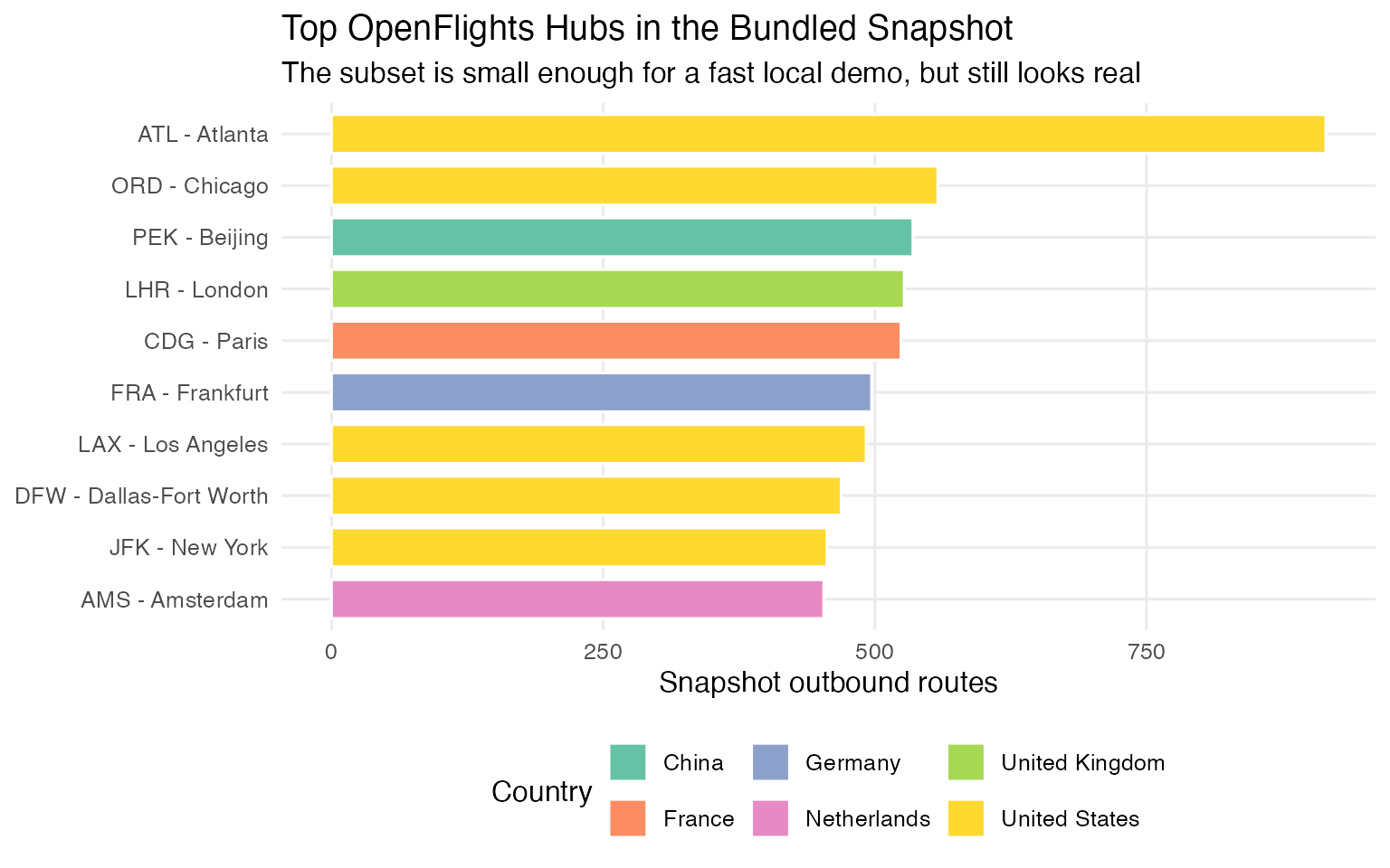
#> 56 12Visualize the hubs
top_hubs <- airports_tbl[seq_len(min(10L, nrow(airports_tbl))), , drop = FALSE]
top_hubs$airport <- factor(
  paste(top_hubs$a.iata, top_hubs$a.city, sep = " - "),
  levels = rev(paste(top_hubs$a.iata, top_hubs$a.city, sep = " - "))
)

ggplot(
  top_hubs,
  aes(
    x = airport,
    y = a.snapshot_outbound_routes,
    fill = a.country
  )
) +
  geom_col(width = 0.75, color = "white") +
  coord_flip() +
  scale_fill_brewer(palette = "Set2") +
  labs(
    title = "Top OpenFlights Hubs in the Bundled Snapshot",
    subtitle = "The subset is small enough for a fast local demo, but still looks real",
    x = NULL,
    y = "Snapshot outbound routes",
    fill = "Country"
  ) +
  theme_minimal(base_size = 12) +
  theme(
    panel.grid.minor = element_blank(),
    legend.position = "bottom"
  )
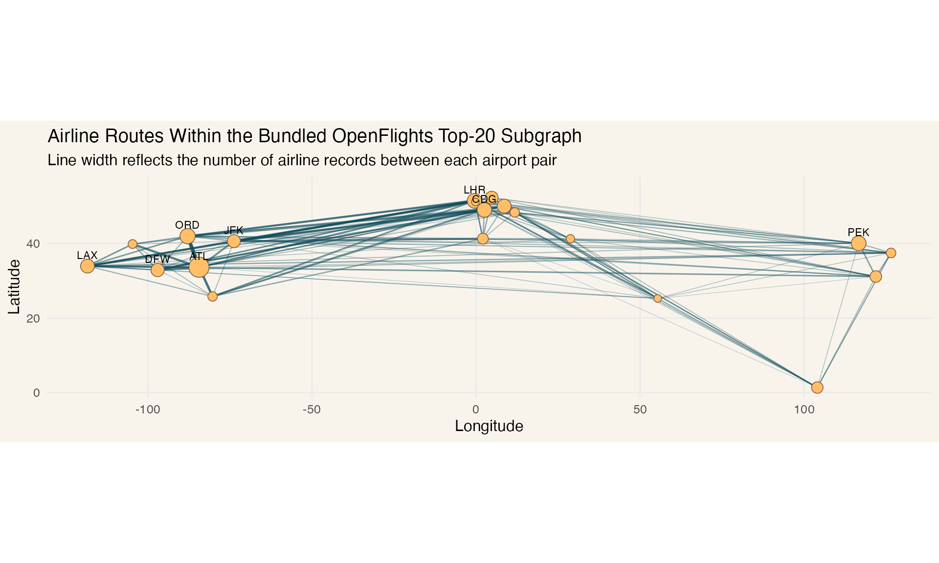
Visualize the route network
labels <- airports_tbl[seq_len(min(10L, nrow(airports_tbl))), , drop = FALSE]

ggplot() +
  geom_segment(
    data = route_segments,
    aes(
      x = source_lng,
      y = source_lat,
      xend = dest_lng,
      yend = dest_lat,
      linewidth = airline_count,
      alpha = airline_count
    ),
    color = "#0f4c5c",
    lineend = "round"
  ) +
  geom_point(
    data = airports_tbl,
    aes(
      x = a.lng,
      y = a.lat,
      size = a.snapshot_outbound_routes
    ),
    shape = 21,
    fill = "#ffbf69",
    color = "#7f5539",
    stroke = 0.4
  ) +
  geom_text(
    data = labels,
    aes(
      x = a.lng,
      y = a.lat,
      label = a.iata
    ),
    size = 3,
    nudge_y = 3,
    check_overlap = TRUE
  ) +
  coord_quickmap() +
  scale_linewidth(range = c(0.2, 1.3), guide = "none") +
  scale_alpha(range = c(0.15, 0.7), guide = "none") +
  scale_size(range = c(2.5, 7), guide = "none") +
  labs(
    title = "Airline Routes Within the Bundled OpenFlights Top-20 Subgraph",
    subtitle = "Line width reflects the number of airline records between each airport pair",
    x = "Longitude",
    y = "Latitude"
  ) +
  theme_minimal(base_size = 12) +
  theme(
    panel.grid.minor = element_blank(),
    plot.background = element_rect(fill = "#f8f4ec", color = NA),
    panel.background = element_rect(fill = "#f8f4ec", color = NA)
  )
The bundled sample is documented in
inst/extdata/openflights-README.md, including the upstream
source URLs and license attribution to OpenFlights.